High-Flow Field Experiments to Inform Everglades Restoration: Experimental Data 2010 to 2016

Benchmark Elevation Surveying: Minor variations in topography are important drivers of sheet flow in the extremely flat terrain of the Everglades. Traditional ground-based surveying is impractical in the DPM research area as a result of the long distances involved, the challenging water-covered environment and the soft sediment conditions. A satellite-based survey was conducted to establish benchmark elevations at most of the DPM research sites in order to determine ground elevations and to relate the measured water levels across the project area to a common elevation datum. Static surveys were performed using Global Navigation Satellite Systems (GNSS) techniques following general guidance (Rydlund and Densmore, 2012) to achieve Level 1 precision, i.e., the highest quality with the lowest achievable uncertainty. Surveys were conducted three times between 2012 and 2015. Elevations were determined in the NAVD 1998 datum of fixed benchmarks that were installed near the platforms at DPM sites Z51_USGS, RS1D, RS2, S1, UB1, UB2, UB3, DB2, C1, and C2. Each survey consisted of two four-hour static deployments, one each day, with the first deployment in the morning the first day and the second during the afternoon the second day to collect data from a different set of satellites during each survey. Data files were submitted to NGS Online Positioning User Service (OPUS) program for processing. Differential gaging station leveling techniques (Kenney, 2010) were used to transfer the NAVD 88 elevation from the monument to the other reference markers at DPM research sites.

Microtopography: Small-scale topography variations (referred to as microtopography) were measured at various sites, focusing on determining the surface elevations of the flocculent organic surface of the wetland and the underlying consolidated peat along ridge to slough transects. This was accomplished by repeatedly collecting measurements of the depth from the water surface to the surface of the floc and peat, and then relating the surface water elevation to a local surveyed elevation. The water depths to floc and peat, hfloc,and hpeat, are measured by determining the vertical distance from the water surface to the floc and peat using a calibrated CPVC depth probe with an I-shaped foot, as described in Choi and Harvey (2013). The probe was gently placed on the floc to measure the depth to floc, and then pressure was applied to sink the probe through the floc in order to measure the depth to peat. In 2010 and 2011, measurements were made at approximately 30 points, oriented in a large circle with a radius of roughly 100 m. At each of the 30 locations, 6 microtopography measurements were taken (6 floc surface elevations and 6 corresponding peat surface elevations). The position of the circle was chosen to include both ridge and slough topographies. Additionally, from 2010 to 2016, water depth to floc and water depth to peat measurements were collected near the study sites, as well as along ridge to slough transects at each site. Three measurements were collected within one square meter at each sampling point to calculate an average water depth to the floc and to the peat. The elevations of the ground surfaces, with subscript floc indicating the flocculent organic matter surface and peat indicating the consolidated peat surface, e.g., Zfloc or Zpeat, respectively, were found by subtracting the measured water depth to the floc or peat (hfloc or hpeat) from the surface water elevation (ZWL ) at the site for a given day and time (Refer to Documentation to Eq-1 and Eq-2).

Surface Water and Groundwater Levels: Surface water levels were obtained using methods suggested by the USGS Office of Surface Water (Kenney, 2010) using pressure transducers with an accuracy of +/- 0.3 cm and that record water level at 5-15 minute intervals. Pressure transducers (KPSI 501 series) were deployed by emplacement in 1.5 inch PVC standpipes. The PVC standpipes were affixed with a through-bolt to a steel pipe previously driven into the bedrock. The reference marker (RM) is located at the top of the steel pipe, and the reference markers are surveyed for the elevation (ZRM) by GNSS technique. Pressure transducer sensors were suspended within standpipes at a pre-determined height where the hole on the side of each sensor was close enough to the ground surface that surface water could always enter the hole, even at very low water levels. The elevation of the KPSI pressure transducer sensor (ZKPSI) is determined by relating the RM elevation and measured distance between RM to KPSI senor. KPSI transducer-measured water levels, ZWL-KPSI, were calculated by adding transducer hydrostatic pressure readings, HPKPSI, to the transducer reference elevation, ZKPSI (Refer to Documentation Eq-3). Another alternate measurement of surface water elevation using reference markers were made during site visits to serve as checks on the measurements of surface water elevation using KPSI transducers. These discrete measurements of a reference surface water elevation, (ZWL-RM), were made by measuring as the vertical distance from the top of the reference steel pipe (RM) down to the surface of the water, which is referred to as a down to water measurement (DTW). DTW measurements were subtracted from the elevation of the top of the reference mark (ZRM) to determine a reference water elevation (ZWL-RM) (Refer to Documentation Eq-4). The reference water levels are independent of pressure transducer data and therefore serve as a check on pressure transducer measurements. Transducer-measured water levels were compared with reference water levels to account for offset and drift of transducers. Over time the expected slope of ZWL-KPSI measurements plotted versus ZWL-RM measurements is expected to be 1 with an intercept of zero. On a given site visit no adjustment was made unless the difference of ZWL-KPSI and ZWL-RM was greater than 0.7 cm. If the difference was greater, an average of the offset measured during that visit and the offset measured during the previous visit was used for the time period between visits. USGS data on water levels from EDEN-8 (located in WCA-3A), TI-9 (located in WCA-3B), and water levels from the S-152 Headwater and S-152 Tailwater sites were included for comparison with DPM water levels. Pressure transducers were installed at sites C1, C2, DB2, MB2, Z51_USGS, RS1D, RS2, S1, UB1, UB2 and UB3. Additionally, three sites, Z51_USGS, RS1 and UB2, had groundwater transducers installed. Groundwater transducers collected data in 15-minute intervals. Data were downloaded and instrument diagnostics performed at approximately monthly intervals. Surface water transducers began deployment in October 2010 and will remain deployed for the duration of the DPM project. Groundwater transducers were installed in November 2012 and will also remain deployed for the remainder of the project. Groundwater-surface water interactions were assessed by measuring the vertical hydraulic gradient, dh/dL, through the peat layer, where previously they were observed with environmental tracers and seepage meters (Harvey et al. 2004). To calculate the gradient, the measured reference elevation of surface water (ZWL-RM,sw) from the elevation of the groundwater (ZWL-RM,gw) and dividing that difference by the vertical distance (L) from the center of the screen of the piezometer emplaced in the peat to the peat surface (Refer to Documentation Eq-5). As defined, the hydraulic gradient expresses groundwater recharge as a positive value and discharge as a negative value. Reference groundwater elevations are determined by measuring DTW inside the groundwater piezometer at the time of site visits. Hydraulic gradients were also analyzed using transducer-measured water levels (ZWL-KPSI,sw and ZWL-KPSI,gw), with careful consideration given to correct transducer offset and drift to achieve the needed accuracy.

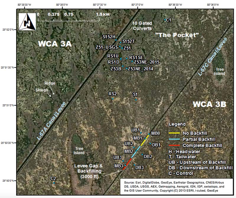
Surface Water Flow Velocities and Shear Stress: Flow velocity was measured in surface water at the main monitoring sites (C1, C2, Z51_USGS, RS1D, RS2, S1, UB1, UB2, UB3, DB1, DB2, DB3, MB0, MB1, and MB2) that were selected to overlap with other hydrologic and biogeochemical measurements (fig 1). Flow velocity was measured by 10 megahertz [MHz] up/down/side-looking Acoustic Doppler Velocimeters (ADV) manufactured by SonTek/YSI and by Vectrinos manufactured by Nortek. In the canal sites, MB1 and MB2, Autonomous Argonaut XRs were deployed (manufactured by SonTek). The ADV and Vectrino approach can measure flow velocity to a resolution of 0.01 cm/s and 0.1 cm/s with an accuracy of 1% and 0.5% of measured velocity, respectively (SonTek, 2001). The general operating procedure for ADVs outlined in Harvey et al. (2009) was followed for data collection. Continuous velocities were collected from a fixed depth at approximately the midpoint of the water column at a frequency of 10 Hz. ADV flow velocity data were recorded in one minute bursts (600 samples), and collected every 15 minutes to save battery power. Velocity datasets were filtered and edited according to standard criteria suggested by the instrument manufacturer (SonTek, 2001) as well as specific criteria developed and refined in a prior Everglades study (Riscassi and Schaffranek, 2002). To ensure data quality, ADV data had to pass a 40% minimum correlation filter with at least 70% of samples within a burst being retained (Martin et al., 2002). Data with an acoustic signal-to-noise ratio (SNR) of 5 dB or less were discarded. The ADV data collected during times when the boats were known to be present at the monitoring sites were removed. A sound-speed correction was applied to ADV data using either data from an attached Convention Temperature Device (CTD) or average temperature and salinity recorded by a nearby CTD during the deployment period. The Vectrinos also applied a sound-speed correction using an embedded thermistor and measured salinity. The 3-dimensional velocity data underwent a rotation for magnetic declination, as ADVs and Vectrinos were deployed such that the positive x-velocity direction was oriented to the direction of magnetic north. Finally, a phase space threshold despiking algorithm (Goring and Nikora, 2002) was applied to both ADV and Vectrino data. The resulting quality-assured data were used to produce hourly and daily values and statistics. Calculations of standard deviation of flow direction were performed using the Yamartino method (Yamartino, 1984). ADVs were serviced during continuous deployments, during which data were downloaded, batteries were replaced, the compass was calibrated and diagnostics were performed on the instrument. Between site visits, the height of the ADV sensor was adjusted to keep the sensor submerged until the next site visit. The height of each ADV sensor was adjusted to keep the sampling volume approximately at or slightly below the middle depth of the water column anticipated for the deployment period. ADVs were deployed on average for sixth months in 2010-2014 water years, centered on the operational window for flow releases (November and December). Velocity profiles were measured vertically in the water column using Sontek ADVs as described in Harvey et al. (2009), during most monthly site visits by adjusting the height of the ADV sensors deployed for continuous monitoring. Nortek Vectrino instruments were used to measure velocity profiles at discrete sites. For the profiles, velocities were measured at 10 Hz in 1 minute bursts yielding 600 samples at each depth increment. Flow velocities were measured at 2-5 cm depth increments throughout the water column, depending on total water depth, apparent vertical variability in vegetation architecture, and overall favorability of measurement conditions and time constraints. Signal-to-noise-ratios were monitored continuously during collection of the vertical velocity profiles to determine if the sample volume was obstructed by vegetation and as an indicator of the vertical location of the top of the floc. Velocity profile data underwent the same corrections and filters as the continuous velocity data. In some cases, bursts in which fewer than 70% of samples passed the 40% correlation filter were retained if the data seemed reasonable, in order to avoid complete elimination of useful data. The large number of samples averaged for each burst and the filtering and quality assurance procedures used to edit and process the data provided confidence that the maximum possible resolution (0.01 cm s-1) reported for this instrumentation (SonTek, 2001) was achieved in these measurements. Discrete velocities were sampled along vertical water column profiles with a Sontek ADV FlowTracker at sites where no continuous ADV data were collected and where use of a Nortek Vectrino was impractical. The FlowTracker approach can measure flow velocity to a resolution of 0.01 cm/s with an accuracy of 1% of measured velocity (SonTek, 2001). Data were recorded in one minute bursts collected at different depths; low (5cm above floc surface), middle of the water column and upper (5cm below water surface). The FlowTracker was positioned in a location with approximately 30cm of clear space around the sensor and vegetation was clipped if necessary. The operating procedure performed was followed according to the FlowTracker Handheld ADV Technical Manual (2007) and post-processing QA/QC followed the procedures described above for the ADVs. For the velocity at the canal, acoustic doppler profilers (Argonaut-XRs) were deployed at MB0, MB1 and MB2 (Figure 1) to provide continuous records of velocity profiles. The Argonaut-XR approach can measure flow velocity to a resolution of 0.1 cm/s and 0.1 cm/s with an accuracy of 1% of measured velocity, respectively (SonTek, 2001). Argonaut-XRs were deployed in an up-looking configuration and sample vertical profiles of flow speed and direction in one-minute bursts collected every 15 minutes. Post-processing QA/QC followed the procedures described above for the ADVs. Depth-averaged flow velocities were computed directly from the profiles. A step not yet accomplished that could improve estimates is to relate instantaneously measured velocity profiles to long-term data collected at a single point in the water column. Essentially, point velocities can be converted to depth-averaged velocities using velocity profile shape factors described in the procedures documented in Lightbody and Nepf (2007) and in Harvey et al. (2009). Bed shear stress measurements were taken pre-release and during the flow release at 6 discrete points along the RS1U ridge-to-slough transect using a Vectrino II Profiler ADV, manufactured by Nortek. To compute bed shear stress, a Vectrino Profiler was mounted on a vertically sliding rod and deployed to sample flow immediately above the bed. Each instrument reading consisted of instantaneous velocity collected over 18 points within a 2.5-cm vertical profile, at a spacing of 2.0 mm. The instrument was operated at high power to achieve the maximum signal-to-noise ratio, with pinging set to max interval. Each reading was acquired over a period of 5 minutes. At the end of 5 minutes, the profiler was moved to its next location along the sliding rod (which overlapped with the first by about 0.5 cm) and again deployed. In this manner, four stacked 2.5-cm profiles were obtained near the bed. A fifth 2.5-cm profile was acquired in the middle of the water column at each site. Raw velocity records were filtered to remove data points that did not meet standards for signal-to-noise ratio (at least 5 dB), correlation (at least 40%), or consistency in redundant measurements of the z-direction velocity component. Instrument noise spikes were removed using Goring and Nikora’s (2002) threshold despiking algorithm. Following Biron et al. (2004), profiles of total stress were calculated as the sum of the total kinetic energy derived stress and laminar stress (Refer to Documentation Eq-6). The maximum near-bed total stress was selected as the bed shear stress.

Suspended Particle Sizes and Concentrations: During both DPM flow releases in 2013, 2014, and 2015, samples were collected for analysis of suspended sediment concentration (SSC), SSC load, suspended particle size, and associated total phosphorus (TP) concentration and TP load. Water column samples were collected by peristaltic pumping at a rate of 60 ml/min through size 16 Masterflex tubing with a 500 μm Nitex screen fitted to tubing inlet. Two liters sample was collected for SSC analysis, 250mL was collected to be run in the field on the LISST-Portable, and a 60ml sample was collected for TP analysis which was preserved with H2SO4 at a pH of 2 and placed on ice before shipment to the South Florida Water Management District Lab. During the DPM high flow event beginning in November 2013 the water column samples were collected at sites RS1U, UB1, UB2, S1, DB1, DB2 and DB3 prior to the high flow (before 09:40 11/5/2013), during the flow breakthrough (09:40 11/5/2013 –11/6/2013), and during the steady high flow that followed (11/7-8/2013, 11/10/2013). During the DPM high flow event beginning in November 2014 the water column samples were collected at sites RS1U, RS1D, Z53B, RS2, S1, UB1, UB2, UB3, DB1, DB2, DB3, RS1SE, Z51 and S-152 prior to the high flow (before 09:43 11/4/2014), during the flow breakthrough (09:43 11/4/2014 – 11/5/2014), and during the steady high flow (11/7/2014, 12/4/2014, 1/21/2015) and after the closing of S-152 (3/9-10/2015). During the DPM high flow event beginning in November 2015, the water column samples were collected at sites Z51_USGS, RS1D, RS1SE, UB1, UB2, UB3, DB1, DB2, DB3 (before 09:40 11/16/2016, 12/9/2015, 1/20/2016, and 3/2/2016). During the two pulsed high-flow period, the water column samples were collected at sites Z51_USGS, RS1D, and RS1SE (09:40 to 17:00 11/16/2015, 9:00 to 17:00 11/17/2015, 09:40 to 17:00 11/19/2015, 9:00 to 17:00 11/20/2015). Site names beginning with RS had paired sampling from nearby ridge and slough. At other sites samples were collected from only sloughs. At RS1U samples were collected at 2-meter spaced intervals across the transition between ridge and slough. At the transect endpoints in the ridge and slough the samples were collected to represent the upper third, middle, and near-bed water (5cm above floc surface) water column. At RS1U locations between the transect endpoints only near-bed samples were collected. Samples from the upper water column were omitted in 2014. In 2014 sites RS1D, Z53B, RS1SE and RS2 were sampled from the low and middle water column in the ridge and slough. At slough sites Z51_USGS, S1, UB1, UB2, UB3, DB1, DB2 and DB3, samples were collected from only the low and middle water column. In the laboratory the volume of each suspended sediment sample was measured prior to filtration with a graduated cylinder. Each sample was then processed by vacuum filtration through a 0.7 μm filter (Whatman GF/F) (Noe et al., 2010). Filters were prepared by vacuum filtering 100mL of deionized water through the filter and then heating at 500°C for one hour to remove any present organic material. The initial dry mass of the filter was measured on an analytical balance. The sediment laden filters were oven dried at 60°C and then weighed with an analytical balance. With this information, suspended sediment concentration was calculated for each sampling time at each site by subtracting the mass of the dried filter from the mass of the sediment laden filter and dividing the difference by the volume of the sample. Duplicate SSC and TP samples were collected on 11/5/13 at two locations (sites RS1U_RR-M and RS1U_SS-M) and on 11/8/13 at two locations (sites S1_L and UB1_L). They were also collected at sites RS1U_RR-M and RS1U_SS-M on 3/10/2015 and UB2 and DB2 on 3/9/2015. Duplicate samples were analyzed to determine the amount of error present within sampling and processing methods. Total phosphorus concentrations (TP) of the water column samples were analyzed by the South Florida Water Management District Lab by first subjecting the samples to an acid-persulfate digestion to convert organic and inorganic phosphates into reactive phosphate. Total Phosphorus analysis is based on the formation of a blue-colored antimony-phosphomolybdate complex from the reaction of ammonium molybdate, and antimony potassium tartrate with reactive phosphate in an acidic medium followed by reduction with ascorbic acid. The blue color complex is measure by photometric analysis at 880 nm on the Lachat Flow Injection Analyzer (FIA) with a detection limit of 0.002 mg/L and detection range of 0.002 to 0.4 mg/L. The total phosphorus concentration includes phosphorus associated with sediment and dissolved in the water column. Depth-averaged values of SSC and TP concentration were calculated at locations where vertical sampling was conducted in the water column. The total water depth was divided into water column intervals (WCIi) where subscript i is a counter for water column intervals for which there were as many as the number of samples collected vertically in the water column. The WCIi for a given sample was determined by summing the vertically measured half-distances to the adjacent samples above and below (or the whole distance if the sample in question is the nearest to the floc surface or water surface) (Refer to Documentation Eq-7). Depth-averaged SSC and TP concentrations were analyzed spatially to determine distribution variation across the study area. Distances were calculated as a nominal distance along the predicted flow path. To simplify the analysis, the primary flow path direction was chosen as a linear path from the S-152 culverts to site MB2, another linear path segment from site MB2 through site DB2. Site locations were perpendicularly projected to the primary flow path to calculate the nominal distance from the S-152 culverts. The flux of SSC and TP per unit cross sectional area of wetland was determined using velocity data collected by either a Sontek ADV or Nortek Vectrino at each sampling location and water depth where SSC was sampled. If multiple flow velocities had been measured within a water column interval, the depth-averaged velocity within that interval was applied (Refer to Documentation Eq-8 and 9). The same approach for load calculations was applied for TP as for SSC. The direction of the depth-averaged load was calculated using depth-averaged east- and north-components of flow velocity and depth-averaged concentration of SSC and TP, which allows loads to be displayed as vectors. Water column samples collected by the same method and at the same time as samples for SSC and TP were analyzed in the field to determine suspended particle size. A LISST-Portable benchtop laser diffraction particle size analyzer (Seqouia Scientific) was used to optically analyze suspended sediment to produce size distributions across a range from 0.34 - 500 μm. This instrument has a resolution of <1 mg/l an accuracy of ± 20% of measured concentration. The Three to five sample runs were averaged to determine the average particle size distribution. The analyzer also computed metrics such as median volume-weighted, D50 which is the grain diameter at which 50% of the sediment sample is finer. Sediment sizes D10 and D60 were also computed to quantify the 10% and 60% finer than fractions. A particle size uniformity coefficient, D60/D10, was calculated with larger values of D60/D10 indicating a more poorly sorted suspended sediment sample. Depth-averaged values for D50 and D60/D10 were calculated with the same using the same procedure to calculate depth-averaged SSC values. Continuous records (on the order of days) of suspended particle size distributions were obtained at a single site using a laser diffraction particle size analyzer (LISST-100X or LISST-FLOC, Sequoia Scientific) as described in Noe et al. (2010) and Harvey et al. (2011). The Sequoia LISST instruments emit light and measure laser diffraction to estimate the in situ volume concentration and size distribution of particulates in suspension. The particle size measurement range is 1.25 - 250 μm and 7.5 - 1500 μm for the LISST-100X and LISST-FLOC, respectively, and the ranges are analyzed by dividing into 32 logarithmically spaced size-class bins. The resolution of LISST-100X and LISST-Floc is less than 1mg/L. The instruments are deployed horizontally at the mid-point of the water column and programmed to collect data in 60-second bursts every 15 minutes. The instruments can be subject to biofouling, which limits deployment to periods of up to three days. All outputs of LISST particle size distributions from the several different instrument models are volume-weighted. To convert volume-weighted to mass-weighted values, a particle density distribution was applied to the LISST output based on a settling column experiment using Stoke’s Law to compute particle density as a function of particle size as described in Larsen et al. (2009a) and implemented in Harvey et al. (2011).

Biogeochemical Sampling: Water column, metaphyton (i.e., epiphyton and floating periphyton), and bed floc samples were collected and analyzed for particulate phosphorus, organic content, and particle size. Water column samples were collected using a peristaltic pump from the mid-point of the water column. Metaphyton samples were collected using a wet/dry vacuum to collect epiphyton from vegetation stems and periphyton at mid-water depth, as described in Larsen et al. (2009a). Bed floc samples were collected by coring the floc/peat, allowing the sample to settle, pouring off any clear liquid, and then retaining the remaining suspended sample (floc). Water column, floc and metaphyton samples were passed through 500 μm Nitex filter prior to being stored on ice and were shipped either the same day or the next day to the analytical laboratory. Particle size analyses were performed in the field on a LISST-Portable benchtop laser diffraction particle size analyzer (Sequoia Scientific) as previously described. Samples were shipped over night to the Wetland Biological Laboratory, University of Florida, Gainesville, FL in coolers containing wet ice to maintain a sample temperature of 4°C. The following biogeochemical analyses were performed: dry weight of solids, loss on ignition (LOI), total nitrogen (TN), total phosphorus (TP) digestion and analysis, NaHCO3 extraction, and NaHCO3 plus chloroform extraction. For dry weight, samples were dried to a constant weight (detection limit of 0.01%), and for LOI, samples were ignited at 550±50°C in a muffle furnace. Weights were determined using scales and balances verified daily using NIST certified weights. TN was found using a Thermo Electron FlashEA 1112. Samples for TP underwent a perchloric acid digestion and were analyzed using a Technicon Autoanalyzer AA3. The results from NaHCO3 and NaHCO3 plus chloroform extraction were used to determine organic phosphorus fractions consisting of refractory, microbial and labile phosphorus (Ivanoff et al., 1998) (Refer to Documentation Eq-10 to 15).

Vegetation Influence on Sheet Flow: Vegetation community structure is an important factor affecting the shape of velocity profiles, in determining the distribution of velocities close to the bed and in measuring entrainment and transport of suspended sediment (Harvey et al. 2009; Larsen et al., 2009b). Therefore, vegetation community composition, biomass (biovolume, including separate analysis of periphyton), and stem densities were determined by harvesting of vegetation in 0.25 m2 clip plots and measuring the distribution of stem diameters and frontal areas (Harvey et al., 2009; Lightbody and Nepf, 2006). Within a desired sampling area the vegetation quadrats were positioned using a stratified random sampling scheme at ridge, slough, and transition zones at all sites within the hydrologic monitoring network. Once the quadrats were situated the vegetation above the water surface was clipped and bagged as one sampling increment. Below the water surface, vegetation was sampled in 10 cm increments from 2010 - 2012 and 15 cm increments from 2013 - 2014 proceeding from the water surface to the sediment water interface. Sample increments intersecting the bed were clipped at the floc surface, bagged, and stored in the dark and on ice for transport to the laboratory for further processing. In the lab, sample increments were spread out and categorized by species. Measurements of stem diameter and length were collected for the purpose of calculating the average diameter and the frontal area of stems, i.e. the exposed area of stem per unit volume in the water column. First the number of stems and leaves were counted for Cephalanthus occidentalis, Cladium jamaicense, Justicia angusta, Nymphaea odorata, and Panicum hemitomon. The width of 10 randomly selected stems were measured for each species, with width being measured as the distance across the middle of each stem fragment along the widest dimension (major axis) and across the narrowest dimension (minor axis) as measured using a micrometer. For every leaf (or if there were greater than 10 leaves, 10 were randomly chosen) the width, length and thickness were measured using a ruler or micrometer. Frontal area and dimensional volume were then calculated (Refer to Documentation Eq-16 to 18). Vegetation measurements were made repeatedly during the years of experimentation to establish a record of temporal variation related to seasonal and interannual variations and fire. Vegetation-flow relationships are being determined to verify empirical predictive relationships between biomass and flow resistance parameters used in hydraulic models (e.g., Harvey et al., 2009). In addition, vegetation measurements were used to help characterize how flow affects key ecological processes such as ecosystem primary production, decomposition, and nutrient cycling.

Water Quality Monitoring: Water quality parameters were monitored to quantify arrival times of conservatively transported environmental tracers and suspended sediment with the water release into the pocket by the opening of the S-152 culverts. Specific conductivity is a potentially useful tracer to quantify the relative speed of the released water in sloughs and ridges and of the rate of mixing between those waters, as well as the transport rate of suspended sediment entrained during transport. During the high flow releases in November 2013 and November 2014 continuous measurements of specific conductivity and turbidity were collected by deploying YSI sondes at selected sites prior to the opening of the culverts and collecting them 4 days later. The turbidity probe has the range of 0 to 1000NTU, resolution of 0.1 NTU, and accuracy of +/- 2%. And the conductivity probe has the range of 0 to 100 mS/cm, resolution of 0.00 to 0.1mS/cm, and accuracy of +/- 0.5%. Sondes were deployed at sites RS1U_S, S1, UB1, DB1, DB2, and DB3 in 2013 and Z-51_USGS, RS1U_S, RS1U_R, RS1D_S, RS1D_R, Z5-3B_S, RS1-SE_S, RS1-SE_R, Z5-3NE_S, and Z5-3NE_R in 2014. Additional data were attained from USGS stations at 3A, S-152 Headwater and Tailwater, and Site 69 East and West for comparison. To install the sondes in the water column, 1.5 inch PVC pipes were placed in the peat and the YSI sondes were attached to the exterior of the pipes such that the sensors were approximately at the midpoint of the water column. Sampling occurred autonomously on five minute intervals. The YSI turbidity probe is an optical probe with an autonomous cleaning mechanism to prevent biofouling. Before deployment, the turbidity probes were checked in deionized water and if they were not reading within +/- 2 NTU, a 3-point calibration was performed. The conductivity probes were checked in 250 μS/cm standard. If values were not within +/- 5 μS/cm, a 1-point calibration was performed. If no calibration was necessary, a 2-point check (50 and 1000 μS/cm) was performed. Immediately before deployment, all sonde readings were checked against one another in south Florida tap water.

Groundwater-Surface Water Interactions Detected using Heat as a Tracer: Groundwater-surface water interactions are often difficult to detect by hydrometric measurements. Vertical water flux through peat can be estimated from observations of the hydraulic head gradient using Darcy’s Law. Vertical flux through a peat also may be detectable by deploying temperature sensors vertically in sediment and modeling heat transport to constrain the vertical flux of water. Traditional piezometers were installed with four temperature sensors in the DPM experimental footprint in the central Everglades at sites RS1D, S, UB2 and Z51-USGS. Each piezometer is made of a 0.5m long and 1 inch wide PVC pipe enclosing four TMCx Water/Soil temperature sensors connected to a single HOBO U-12 4-channel data logger (with resolution 0.02℃ and accuracy ±0.25℃). The piezometer was inserted into the peat with temperature sensors located at the floc-peat interface (0 cm depth) and three additional depths within the peat sediment. Three depth configurations were used. Configuration 1 had probes located at 0, 5,15, and 35 cm below the peat surface. Configuration 2 had probes located at 0, 5, 10, and 15 cm below the peat surface. Configuration 3 varied by site and had a probe at the floc-surface water interface, floc-peat interface (0cm), at half of the peat thickness (69-87cm), and at the deepest possible point given the length of pipe (133-143cm). Each sensor collected temperature every 10 minutes from 9/28/2013 to 3/2/2016. Before installation, measurements in a well-mixed, warm bath were used to compare the accuracy of the sensors. For this controlled experiment, the sensors showed an accuracy of approximately 0.05℃, which is better than the accuracy reported by the manufacturer.